Running a dynamic frequency analysis

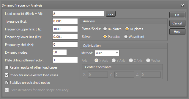
You can run a dynamic frequency analysis by selecting "Dynamic Frequency Analysis" from the Analysis menu.

The dynamic frequency analysis is a linear analysis and hence cannot be used with models that contain cable members. Furthermore, it treats tension-only and compression-only members as normal members that can take tension and compression.

Note that the requirement to save the stiffness matrix during an initial static analysis is no longer required for a dynamic frequency analysis.

Load case list

If you want to analyse all load cases then this field can be left blank, otherwise you should type in a list of load cases (separated by commas or dashes) that you want analysed.

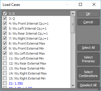
When specifying the load case list, you can either list them directly or you can click the button to display and select from a list of the load cases currently in the job as shown below.

Note that only the load cases that contain lumped masses or self-weight are considered during a dynamic frequency analysis. Any static loads that also exist in the dynamic load cases are ignored.

Consider the following examples:

Self mass

The self mass of the structure is calculated automatically by the dynamic frequency analysis for any load cases that include self weight. Self mass is applied by calculating the mass of each member and then applying half of it as translational lumped masses to each of the member end nodes in each of the unrestrained X, Y and Z global axis directions. The mass of each plate is also calculated and applied to its perimeter nodes

Self mass generation does not calculate rotational masses because of the large number of extra masses that would be calculated for a fairly insignificant improvement in results accuracy. If required, rotational self mass must be manually applied as rotational lumped masses.

See also Lumped masses.

See also Self-weight.

Tolerance (Hz)

The accuracy to which the dynamic natural frequencies will be calculated. For example, a tolerance of 0.001 means that the frequencies will be within +/- 0.001 of the exact value.

The tolerance can also have a significant effect on the accuracy of the mode shapes. While the mode shapes are usually of secondary importance if only a dynamic frequency analysis is done, they are very important if the frequency analysis is followed by a dynamic response analysis. Inaccurate mode shapes from the frequency analysis can cause significant errors in the mass participation factors from the response analysis and its results in general.

Even if a natural frequency is accurate to within 0.01Hz, its corresponding mode shape may not be accurate enough for a dynamic spectral response analysis. If the "Extra iterations for mode shape accuracy" option is turned on (see below) then SPACE GASS will detect significantly incorrect mode shapes during the frequency analysis and will correct them automatically by doing more iterations. Small mode shape inaccuracies cannot be detected by the frequency analysis, however they sometimes make themselves evident in the response analysis by mass participation factors that exceed 100%. A warning is given if this occurs and you should repeat the frequency analysis using a smaller tolerance.

If the results of the frequency analysis won’t be used in a response analysis then a tolerance of 0.01 is more than enough, however if a response analysis is to follow then a tolerance of 0.001 or less should be used.

 Each extra decimal place in the tolerance will increase the number of iterations per mode by 3 or 4. For example, a tolerance of 0.0001 will require 3 or 4 more iterations per mode than a tolerance of 0.001.

Frequency upper limit (Hz)

The upper limit, above which the analysis will no longer search for natural frequencies. Once this limit is reached, the analysis will stop, even if not all requested dynamic modes have been calculated.

Frequency lower limit (Hz)

The lower limit, below which the analysis will skip any natural frequencies found.

Frequency shift (Hz)

The analysis normally calculates natural frequencies starting from 0Hz and working upwards, however if a frequency shift is specified then it starts looking from the frequency shift value instead.

For example, if your structure has natural frequencies of 1.2Hz, 3.2Hz, 3.6Hz, 6.7Hz, 10.2Hz, 15.3Hz and 16.1Hz but you are only interested in the first four frequencies above 3.5Hz, you could specify 4 modes and a frequency shift of 3.5Hz. It would then skip the two lower modes (saving you analysis time) and just find frequencies 3.6Hz, 6.7Hz, 10.2Hz and 15.3Hz.

Dynamic modes

The number of dynamic modes (in ascending frequency order) that are required, starting at the frequency shift value (usually 0Hz). For each mode found, the analysis calculates the mode shape, natural frequency and natural period.

Plate drilling stiffness

Refer to "Plate drilling stiffness" in the static analysis solver.

Retain results of other load cases

If you have specified that not all load cases are to be analysed and, if results already exist for some of the non-specified load cases, you can choose to retain them or have them deleted.

Check for non-existent load cases

If you have defined combination load cases that contain other load cases that don’t yet exist, this option will detect and report them. It is optional because some users prefer to have a standard set of combination load cases that contain primary load cases which are just ignored during the analysis if they don’t exist.

Stabilize unrestrained nodes

Nodes that are free to rotate or translate in one or more directions without resistance from interconnecting members, plates, restraints or constraints can be automatically restrained during the analysis so that instabilities don’t occur.

For example, if a node was connected to a number of members, all of which were pin-ended, a rotational instability would normally result due to the unrestrained rotation of the node. However, the stabilize option would apply a temporary rotational restraint to the node during the analysis, preventing an instability.

Although this solves many instabilities, it doesn’t fix them all, and the prevention of non-trivial instabilities is still dependent on good modelling practice.

Note that if any lumped masses (translation or rotation) have been applied directly to an unstable degree of freedom that has been stabilized with this option, the lumped mass would go into the temporary restraint rather than into the structure. Using the above example again, if a node was connected to a number of members that were all pin-ended and the stabilize option had applied a temporary Z rotational restraint to that node, any Z rotational mass applied directly to that node as a lumped mass would go straight into the temporary restraint rather than into the structure.

Extra iterations for mode shape accuracy

Note that this setting only affects the "Wavefront" and "Watcom" solvers.

The dynamic frequency analysis is complete when the natural frequencies have reached the desired accuracy (as specified by the tolerance), however it is possible that at this point the dynamic mode shapes are not totally accurate. Mode shape accuracy can be achieved by turning on the "Extra iterations for mode shape accuracy" option, however if the dynamic mode shapes are only used as a visual aid to assess the vibration location and its shape then the extra iterations and analysis time involved may not be warranted.

If, however, a dynamic response analysis is to be done based on the frequency analysis then the mode shapes are very important and it is imperative that the "Extra iterations for mode shape accuracy" option is turned on. Even with the extra iterations, in some cases the mode shapes may still not be accurate enough (as sometimes evidenced by a mass participation factor from the response analysis that exceeds 100%) and further accuracy can then only be achieved by using a smaller tolerance.

Plates/Shells

You can choose between "BC" (linear only) elements or "DL" (linear or non-linear) elements. "BC" elements are identical to the ones used in SPACE GASS 12.91 and earlier versions, whereas "DL" elements are new and can be used to model non-linear effects and plate/shell buckling.

"BC" elements use the well known Kirchoff or Mindlin linear plate theories, depending on which type is selected in the input data. They always behave linearly, even during a non-linear static analysis.

"DL" non-linear elements are based on the large-strain/large-deflection version of the Reissner-Mindlin shell theory that takes into account the 2nd order strain terms, stress stiffening, large displacements and large rotations (ie. full large-displacement non-linear theory), whereas "DL" linear elements use a small-displacement/small-strain linear version of the Reissner-Mindlin shell theory. "DL" elements always use Reissner-Mindlin theory regardless of whether you select Kirchoff or Mindlin in the input data.

Because a dynamic frequency analysis is linear, the "BC" Mindlin elements and "DL" elements should produce similar results, although there may be some small differences due to the different theories used.

If you want to perform an analysis that is identical to SPACE GASS 12.91 and earlier versions then you should choose "BC" elements, a drilling stiffness factor of -S (where S is the plate drilling stiffness used in SPACE GASS 12.85, 12.90 or 12.91) and a plate shear thickness that is 6/5 of the shear thickness used in SPACE GASS 12.85, 12.90 or 12.91 (because the shear thickness is now factored by 5/6 internally during the analysis).

Solver

The "Paradise" solver is a new parallel multi-core sparse solver that fully utilizes the multiple cores in a modern computer's CPU. All of the available cores are run in parallel to get the maximum possible analysis speed. It also takes full advantage of the sparseness of the structural matrix during the solution to minimize memory requirements and further increase the speed. Because of its speed, the Paradise solver is the recommended option.

The "Wavefront" solver also takes into account the sparseness of the matrix but doesn't run in multi-core mode. It is generally slower than the Paradise solver and can be used if the Paradise solver is unable to obtain a solution.

Both solvers should yield virtually identical results.

Note that the "Watcom" solver is the one used in pre-SPACE GASS 12 versions. It has been superseded by the Paradise and Wavefront solvers which are both significantly faster.  

Optimization

Refer to "Optimization" in the static analysis solver.

When all of the information has been entered, the dynamic frequency analysis module calculates the natural frequencies, periods and mode shapes for each load case and then saves them ready for graphical or text report output.

If you want to terminate the analysis before it is finished, just press ESC or the right mouse button.