Running a static analysis
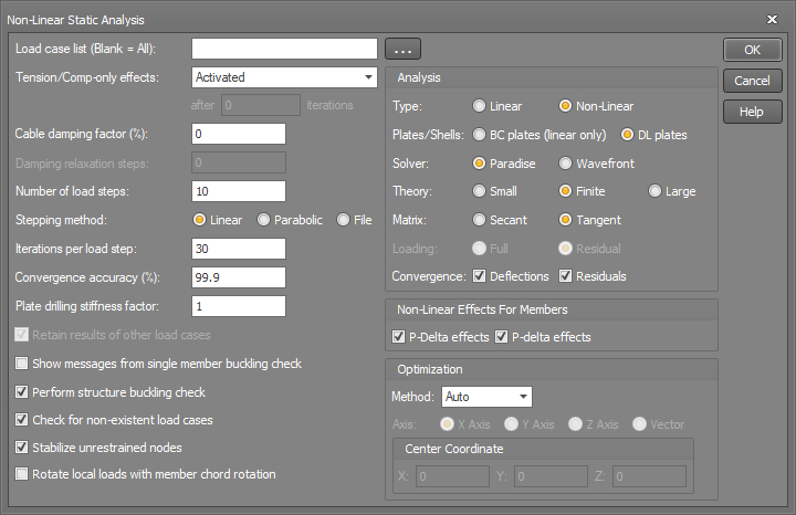
You can run a static analysis by selecting "Linear Static Analysis" or "Non-linear Static Analysis" from the Analysis menu or you can change from linear to non-linear or vice-versa using the Type analysis parameter in the form shown below.
Load case list
If you want to analyse all load cases then this field can be left blank, otherwise you should type in a list of load cases (separated by commas or dashes) that you want analysed.
For the fastest analysis time you should generally analyse only the load cases that can occur in reality. For example, there is no point in analysing a live load case on its own because it can't occur in real life without being combined with dead load. This means that you should generally analyse just the combination load cases and not the primary load cases that the combinations are made from.
It is sometimes also possible to achieve time savings by analysing non-linearly only those load cases that cause 2nd order effects, and analysing all of the other load cases linearly. This would have to be done in two runs, however because a non-linear analysis can take considerably longer than a linear analysis (especially if there are a large number of load cases), it is often worthwhile.
Further time savings can be made by not analysing linear combination load cases. "Linear combination load cases" are combinations that have all of their primary load cases analysed linearly. Results for non-analysed linear combinations are assembled from the primary load cases at the time a report or graphics output is generated. If a combination load case has one or more of its primary load cases analysed non-linearly or if the structure contains tension-only or compression-only members then the combination will have to be analysed in order to obtain results for it.
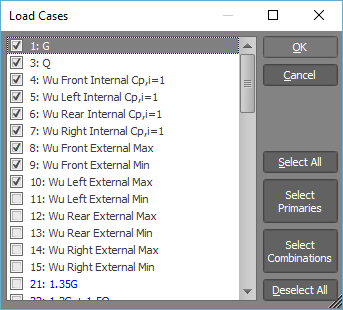
When specifying the load case list, you can either list them directly or you can click the ![]() button to display and select from a
list of the load cases currently in the job as shown below.
button to display and select from a
list of the load cases currently in the job as shown below.
Tension/Comp-only effects
Note that this setting only affects members and not plates/shells.
Tension/compression-only effects can be set to "Activated", "No reversal", "Deactivated" or "Gradually activated".
"Activated" means that tension-only or compression-only members which have been disabled during the analysis are able to be re-enabled if their axial force is reversed.
"No reversal" means that once they have been disabled they cannot be re-enabled even if their axial force has reversed. No reversal is useful if the fully operational analysis will not converge, however you should check the results and, if required, manually disable some tens/comp-only members and then re-analyse.
No reversal normally applies from the first iteration onwards, however you also have the option of activating it after a specified number of iterations. This means that the analysis will initially proceed with tension/compression-only effects fully activated and, if convergence hasn’t been achieved after a specified number iterations, it will change to "no reversal" mode.
You should treat the "No reversal" mode with caution, as it will usually result in members being disabled that would normally take axial load.
"Deactivated" means that they are treated as normal members, able to take tension and compression.
"Gradually activated" means that only the members with large axial loads are disabled in the initial iterations. This is gradually relaxed over a number of iterations until it reverts to the normal "Activated" mode of operation. You can specify how many iterations are involved in the gradual phase. This mode is useful for cases where too many members are initially disabled, causing the model to become unstable before it has a chance to adjust to the disabled members.
See also Tension-only and compression-only effects.
Cable damping factor
This allows you to apply damping to the cable connected nodes. It does this by multiplying the stiffness terms of the unrestrained cable-only node degrees of freedom by the factor:
![]()
where Ratio depends on the damping relaxation and Damping is the cable damping factor.
See also Cable members.
Damping relaxation steps
If cable damping is used, it must be relaxed as the solution proceeds so that at convergence there is no damping at all.
Setting the damping relaxation steps to zero causes the damping to be relaxed in direct proportion to the change in deflection between the current and previous iterations. As convergence approaches 100%, the change in deflections approaches zero and hence the damping approaches zero.
Alternatively, setting the damping relaxation steps to a finite value causes the damping to be relaxed in uniform steps down to zero. If this method is used, the analysis keeps iterating until the damping is fully relaxed, regardless of whether convergence has been achieved earlier or not.
If multiple load steps are specified then the damping relaxation process begins anew for each load step.
See also Cable members.
Number of load steps
Now that non-linear "DL" plates are available, load stepping is much more important than before. Load stepping allows you to apply the load gradually in a number of small load steps. If you specify a single load step then all of the load is applied in the first iteration. The analysis will not finish until all load steps have been completed. For a non-linear analysis with "BC" plates or no plates at all, one load step is usually sufficient, but getting convergence with "DL" plates usually requires more than one load step, and sometimes up to 30 or more.
The analysis time is directly proportional to the number of load steps and so a single step is desirable for maximum speed, however more than one load step is often required when doing a non-linear analysis with "DL" plates or when using finite or large displacement member theory. This is because in those situations a single load step can cause the displacements to overshoot the solution to an extent that further iterations are unable to bring it back to convergence.
It is therefore recommended that for speed you initially try one load step, but if convergence can't be achieved and you are using "DL" plates and/or finite/large displacement member theory then you should try more load steps. For very flexible or sensitive structures you may find that sometimes (but rarely) 50 or more load steps may be required to achieve convergence. To save time you may find that experimenting with the load steps for just a few problem load cases works best, and once you have them working then you can try analysing the full set of load cases. By choosing a different stepping method (see below) you may find that you don't need as many load steps.
The plate drilling stiffness can also affect convergence of non-linear "DL" plates, and so if you are still not getting convergence with a large number of load steps then you should also consider adjusting the drilling stiffness.
Stepping method
When you have specified multiple load steps you can also control whether the steps are applied linearly, parabolically (ie. large steps at first and then gradually smaller) or in some other way that follows a curve or equation. Choosing an appropriate stepping method can help if you are having trouble getting convergence, particularly with models that are very flexible or sensitive to small load increments.
"Linear" stepping is the default and is suitable for most structures. "Parabolic" stepping is intended to roughly follow a typical load-deflection curve that starts off steeply and then gradually levels off as the load approaches the full load. Parabolic stepping may help to get convergence for flexible or sensitive structures if linear stepping can't, particularly with "DL" plates.
If you want to define any general stepping pattern that follows a curve or equation then you can choose the "File" option and define the steps in a text file. This option requires you to create a text file (using any text editor) called "<Job>.@SF" in your temporary data folder (which you can locate via the Settings menu => Storage Folders), where <Job> is the name of your job. When creating or editing the text file you should ensure that you have the job open in SPACE GASS first, otherwise your text file will be deleted or reverted to a previous version when you open the job. This is because the text file gets saved inside the <Job>.SG job file when you close the job and is then restored when you re-open the job.
Each line of the <Job>@SF file should contain "Step, Factor", where "Step" is the step number and "Factor" is the load factor applied to the loads for that step. Each load factor should be within the range of 0.0 < Factor ≤ 1.0. The number of lines in the text file should be no less than the specified number of load steps. If there are more lines than load steps then it will just ignore the extra lines and use a load factor of 1.0 for the final step. For example, a load stepping text file for 10 load steps could contain the following:
1, 0.15
2, 0.30
3, 0.45
4, 0.60
5, 0.70
6, 0.80
7, 0.85
8, 0.90
9, 0.95
10,1.00
Iterations per load step
This parameter allows you to specify the maximum number of iterations that will occur in a load step before the program begins prompting you for extra iterations. More iterations will generally be required when you are doing a non-linear analysis with "DL" plates and/or finite/large displacement member theory. The analysis will finish if the convergence accuracy is satisfied, even if the number of iterations per load step hasn't been completed.
A special case occurs if you specify just one iteration per load step, in which case the program proceeds to the next load step after one iteration regardless of whether convergence has been achieved or not. It is not recommended that you use this option except as a last resort if you are having problems with convergence.
Convergence accuracy (%)
The convergence accuracy is only applicable for non-linear analyses. After each iteration, SPACE GASS compares the results of the latest analysis with the results of the previous analysis. If the comparison shows that the level of convergence has reached or exceeded the specified convergence accuracy then the analysis is assumed to have converged.
If you have tension-only or compression-only members in the model you may sometimes find that the desired convergence % is achieved but the analysis continues iterating for no apparent reason. This is generally because some tension-only members still have compression in them or some compression-only members still have tension in them and so further iterations are required until this is resolved.
If you lower the convergence accuracy, the analysis may not converge sufficiently and you risk getting incorrect results. It is particularly important that you don’t lower the convergence accuracy for highly non-linear structures such as those that contain cables.
Plate drilling stiffness
The rotational stiffness of a plate/shell element about its normal (local z) axis is commonly known as its "drilling stiffness". Plate elements by default have a zero drilling stiffness which can cause instabilities due to the nodes being able to rotate without resistance about the plate's normal axis, unless the nodes are also connected to other plates in a different plane or to members. For example, a horizontal slab supported along an edge by a vertical wall could have unstable nodes in the slab about a vertical axis and unstable nodes in the wall about a horizontal axis, however the nodes that are common to the slab and wall would be not be unstable because the slab and wall elements would prevent each other's unstable rotations.
In order to prevent instabilities due to zero drilling stiffness in plates, a common solution is to apply an artificial drilling stiffness to each plate node using a soft rotational spring. In SPACE GASS this is done automatically to all plate nodes, regardless of what other plates or members they are connected to. To ensure that these rotational springs don't have a significant effect on the results for plate nodes that are also connected to other plates and members that have stiffness about the drilling axis, the drilling stiffness is usually set quite small. SPACE GASS uses a default drilling stiffness that is related to the stiffness of the element to which it is applied. A small stiff plate element will therefore get a larger drilling stiffness than a larger more flexible element. You can increase or decrease the drilling stiffness via the "Plate drilling stiffness factor", where a factor of 1.0 sets the drilling stiffness to its default value. If you don't want any drilling stiffness then you should use a drilling stiffness factor of 0.0, however this may result in instabilities if some plate nodes are then left free to rotate about the plate's normal axis.
The drilling stiffness is calculated according to:
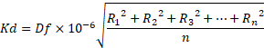
Where Df is the drilling stiffness factor, R1, R 2,..., Rn are the plate's diagonal rotation stiffness terms and n is 12 for a quad element or 9 for a triangular element.
In general, the default drilling stiffness factor Df of 1.0 should work well, but if you get convergence problems, unexplained instabilities or large rotations of nodes about the axes normal to the plates they are connected to then you may have to increase the drilling stiffness factor. You may also find that increasing the drilling stiffness factor can help if the dynamic frequency analysis is unable to find any natural frequencies (eigenvalues). Conversely, you may want to reduce the drilling stiffness if you feel that its default value is too high and the plate node rotations are being over restrained. A simple test is to increase or decrease the drilling stiffness factor to see if the results change significantly. If the results change then you should keep increasing or decreasing the drilling stiffness factor until it gets to a point where further changes don't affect the results significantly. If you can never get to this point then you may be changing the drilling stiffness factor in the wrong direction.
Note that in SPACE GASS 12.85, 12.90 and 12.91 you could only specify the plate drilling stiffness as a torsional stiffness with units of Nmm/rad and a default value of 1.0. It was applied with the same magnitude to every plate element regardless of its size or stiffness. In SPACE GASS 12.80 and earlier versions, the drilling stiffness couldn't be controlled by the user and was hardwired to a value of 0.0001 Nmm/rad. The magnitude of the drilling stiffness doesn't usually have a dramatic affect on the results, but if you are using "BC" plates and want to exactly replicate the results from older versions of SPACE GASS then you can specify a negative plate drilling stiffness factor to have it treated internally as a drilling stiffness with units of Nmm/rad instead of a factor. For example, if you wanted to replicate the results from SPACE GASS 12.85 that had a drilling stiffness of 1.0 Nmm/rad then you could use a drilling stiffness factor of -1.0 or if you wanted to replicate the results from SPACE GASS 12.80 or earlier then you could use a drilling stiffness factor of -0.0001. For "DL" plates the absolute value of the drilling stiffness factor is used and so negating it makes no difference to the results.
If you are comparing "BC" plate results with SPACE GASS 12.91 or earlier then you should also be aware that those older versions relied on you to set the plate's shear thickness to 5/6 of the actual thickness, whereas this is now done internally during the analysis.
Retain results of other load cases
If you have specified that not all load cases are to be analysed and, if results already exist for some of the non-specified load cases, you can choose to retain them or have them deleted.
Show messages from single member buckling check
During a non-linear analysis, SPACE GASS performs a simple Euler buckling check on each member individually (regardless of whether you have the buckling analysis module or not). If the buckling check fails then the member is disabled for the remainder of the analysis. If you select the "Show messages from single member buckling check" check box then a message is displayed whenever a member fails the simple buckling check. For more information, refer to Static analysis buckling.
Perform structure buckling check
SPACE GASS can optionally perform a structure buckling check during a non-linear analysis that simply alerts you if the structure's buckling capacity has been exceeded. If this happens, you cannot use the results of the static analysis because they will most likely be invalid and you should run a full buckling analysis to get the buckling load factor and find out where the buckling is occurring. Note that the structure buckling check is only activated if you choose "Small" displacement theory. For more information, refer to Static analysis buckling and Buckling analysis.
The structure buckling check is very reliable and can be used to verify if the buckling load factors from a buckling analysis are accurate or not, even if the model contains cables. For example, if the buckling analysis of load case 10 produced a buckling load factor of 2.4 and you wanted to verify that this wasn't overestimating the structure's buckling capacity, you could create a new combination load case that factored up load case 10 by close to 2.4 (say 2.3) and then run a non-linear static analysis on it with the structure buckling check turned on. If no buckling message appeared at the end of the analysis then you could be confident that the buckling load factor was at least 2.3.
Note that this check will not include buckling of plates/shells if you use "BC" plates.
Check for non-existent load cases
If you have defined combination load cases that contain other load cases which don’t yet exist, this option will detect and report them. It is optional because some users prefer to have a standard set of combination load cases that contain primary load cases which are just ignored during the analysis if they don’t exist.
Stabilize unrestrained nodes
Nodes that are free to rotate or translate in one or more directions without resistance from interconnecting members, plates, restraints or constraints can be automatically restrained during the analysis so that instabilities don’t occur.
For example, if a node was connected to a number of members, all of which were pin-ended, a rotational instability would normally result due to the unrestrained rotation of the node. However, the stabilize option would apply a temporary rotational restraint to the node during the analysis, preventing an instability.
Although this solves many instabilities, it doesn’t fix them all, and the prevention of non-trivial instabilities is still dependent on good modelling practice.
Note that if any node loads (forces or moments) have been applied directly to an unstable degree of freedom that has been stabilized with this option, the applied node load would go into the temporary restraint rather than into the structure. Using the above example again, if a node was connected to a number of members that were all pin-ended and the stabilize option had applied a temporary Z rotational restraint to that node, any Z moment applied directly to that node as a node load would go straight into the temporary restraint rather than into the structure.
Rotate local loads with member chord rotation
If this option is ticked then after the first analysis iteration any local member loads will be rotated with the chord rotation of the members to which they are applied. It can be used to ensure that wind loads or hydrostatic loads remain normal to the member direction as the model deforms. This option is only enabled with finite or large displacement theory in a non-linear analysis.
Type
Even though you have already chosen "Linear" or "Non-linear" from the Analysis menu, this pair of radio buttons allows you to change your mind without having to exit the form. A linear analysis generally involves only one iteration and does not adjust the stiffness of the structure based on its deformation. It is suitable for simple beams or fully braced frames, but not for sway frames or flexible structures in which non-linear effects are significant. A non-linear analysis involves an iterative procedure that updates the stiffness of the structure after each iteration and gives more realistic results than a linear analysis.
Plates/Shells
You can choose between "BC" (linear only) elements or "DL" (linear or non-linear) elements. "BC" elements are identical to the ones used in SPACE GASS 12.91 and earlier versions, whereas "DL" elements are new and can be used to model non-linear effects and plate/shell buckling.
"BC" elements use the well known Kirchoff or Mindlin linear plate theories, depending on which type is selected in the input data. They always behave linearly, even during a non-linear static analysis.
"DL" non-linear elements are based on the large-strain/large-deflection version of the Reissner-Mindlin shell theory that takes into account the 2nd order strain terms, stress stiffening, large displacements and large rotations (ie. full large-displacement non-linear theory), whereas "DL" linear elements use a small-displacement/small-strain linear version of the Reissner-Mindlin shell theory. "DL" elements always use Reissner-Mindlin theory regardless of whether you select Kirchoff or Mindlin in the input data.
For a linear static analysis you may find that the results are slightly different when comparing "BC" Mindlin elements with "DL" elements, however the differences should not be significant. For a non-linear static analysis they will be very different because the "BC" elements only have linear capabilities.
If you want to perform an analysis that is identical to SPACE GASS 12.91 and earlier versions then you should choose "BC" elements, linear load stepping (if more than one load step), a drilling stiffness factor of -S (where S is the plate drilling stiffness used in SPACE GASS 12.85, 12.90 or 12.91) and a plate shear thickness that is 6/5 of the shear thickness used in SPACE GASS 12.85, 12.90 or 12.91 (because the shear thickness is now factored by 5/6 internally during the analysis).
Solver
The "Paradise" solver is a new parallel multi-core sparse solver that fully utilizes the multiple cores in a modern computer's CPU. All of the available cores are run in parallel to get the maximum possible analysis speed. It also takes full advantage of the sparseness of the structural matrix during the solution to minimize memory requirements and further increase the speed. Because of its speed, the Paradise solver is the recommended option.
The "Wavefront" solver also takes into account the sparseness of the matrix but doesn't run in multi-core mode. It is generally slower than the Paradise solver and can be used if the Paradise solver is unable to obtain a solution.
Both solvers should yield virtually identical results.
Note that the "Watcom" solver is the one used in pre-SPACE GASS 12 versions. It has been superseded by the Paradise and Wavefront solvers which are both significantly faster.
Theory
Note that this setting only affects members and not cables or plates/shells. Cables and "DL" plates in a non-linear analysis always use large displacement theory.
Small displacement theory (based on Ghali and Neville (2)) is the default setting and is suitable for most structures in which the members aren't subjected to significant chord rotations (changes in direction of members). Small displacement theory results are output in the undeformed axes system. The finite and large displacement theories (based on Hancock (24)) take member chord rotations into account and base their equilibrium equations on the deformed geometry. Finite and large displacement theory results are output in the deformed axes system.
Large displacement theory uses more exact methods than finite theory when adjusting the stiffness matrix to allow for the deformation of the structure, however for many structures they produce very similar results.
Note that although the finite and large displacement theories can handle larger displacements, it is often harder to achieve convergence with them than with small displacement theory, especially when large displacements occur. More than one load step is often required to achieve convergence with finite and large displacement theories.
Matrix
Note that this setting only affects members and not plates/shells. "DL" plates in a non-linear analysis always use a tangent stiffness matrix.
The main stiffness matrix can be a secant matrix (relating the full loads to the total displacements) or a tangent matrix (relating the residual loads to incremental displacements). A tangent matrix generally reaches convergence in a smaller number of iterations than a secant matrix and is more suited to large displacements, however this is not always the case. They both yield similar results. Note that small displacement theory always uses a secant matrix.
Residual loads are the imbalance between the applied loads and the internal structural forces at each node. Incremental displacements are the difference in displacements between the current and the previous iteration. The residual loads and the incremental displacements both approach zero as the solution approaches convergence.
Note that if you use a secant matrix with finite or large displacement theory and full loading, the stiffness matrix is non-symmetrical. This means that during the analysis, the stiffness matrix uses up twice as much memory as it otherwise would and so it should be avoided if your model is large.
Loading
Note that this setting only affects members and not plates/shells. "DL" plates in a non-linear analysis always use residual loading.
For a secant matrix, you can choose between full or residual loading (see above), whereas the tangent matrix always uses residual loading. They both yield similar results, but if convergence is a problem then it may be worth experimenting with this setting.
Convergence
Convergence can be based on deflections or residuals or both and is achieved when they approach zero. It is recommended to have them both selected.
P-Delta (P- D) effects
Note that this setting only affects members and not plates/shells. "DL" plates in a non-linear analysis are always fully non-linear and include p-delta effects.
For a non-linear analysis, you are able to activate or de-activate P- D effects for members. The P- D effect is usually the most significant 2nd order effect and is mandatory for non-linear analyses which comply with most limit states design codes of practice. See also P-D effect.
P-delta (P- d) effects
Note that this setting only affects members and not plates/shells. "DL" plates in a non-linear analysis are always fully non-linear and include p-delta effects.
For a non-linear analysis, you are able to activate or de-activate P- d effects for members. The P- d effect is mandatory for non-linear analyses which comply with most limit states design codes of practice. See also P-d effect.
Optimization
The Paradise solver now uses a compressed stiffness matrix which bypasses the optimization step because it is no longer required.
For the Wavefront solver, the optimizer settings are important because they can reduce the analysis time and the required memory. The optimizer can be de-activated or it can be operated in one of four modes as follows.
-
No optimization
-
Auto mode - SPACE GASS trials the "General" and various "Linear" modes and then uses the one that gives the smallest matrix size. It doesn't add significant time to the analysis and is the recommended setting.
-
General mode - SPACE GASS determines the path along which optimization proceeds through the structure.
-
Linear mode - You select from the X, Y or Z axes or a vector along which optimization proceeds in a straight line through the structure.
-
Circular mode - You select either of the X, Y or Z axes about which optimization proceeds around an arc through the structure.
Optimization axis
If you have selected "Linear" or "Circular" for the optimization mode then you must select the axis or vector along or about which optimization will proceed.
Coordinates of optimization centre
If you have selected "Circular" for the optimization mode then you must select the centre of rotation about which optimization will proceed.
When all of the information has been entered, the static analysis calculates the displacements, forces, moments and reactions for each load case and then saves them ready for graphical or text report output.
If you want to terminate the analysis before it is finished, just press ESC or the right mouse button. If you terminate the analysis in this way, the results for any load cases which have already converged are saved.